Visual Search using Deep Learning (pt. 2) - Building the model
Now that we have our labelled dataset ready, let us begin implementing our network.
Understanding the model
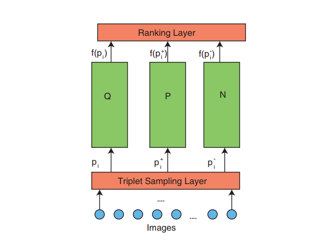
The above diagram is a high level diagram of the network. In the last part of this tutorial, we have built the triplet sampling layer. We will now implement the rest.
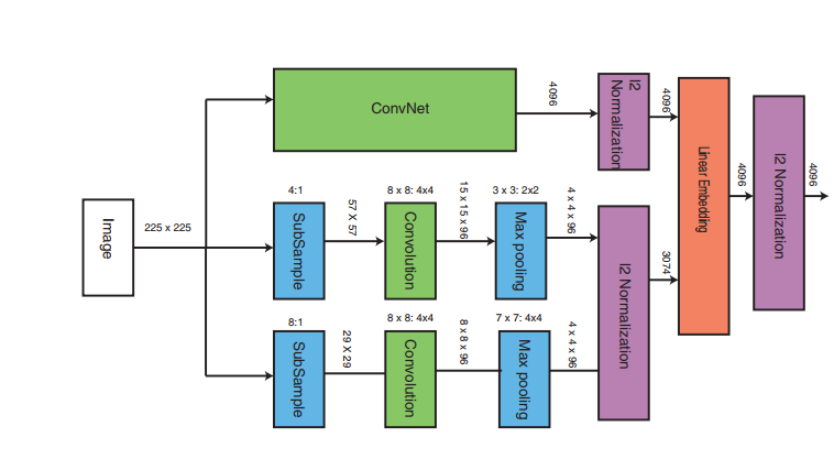
The second diagram is the actual architecture of the Q,P and N blocks in the previous diagram. The ConvNet, in this implementation is a pretrained VGG-16 network.
The intuition behind having propogating the same image through these 3 networks (VGG-16 and shallow networks) is very simple.
- The VGG-16 is capable of picking up and embedding high level visual similarities features while
- the shallow networks can pick up and generate an embedding of low level (coarse) visual similarity features.
The embeddings of these 3 sub-models (VGG-16 and shallow networks) are concatenated to generate the final embedding (4096 bit).
Once our model has learnt an intelligent way to generate embeddings such that embeddings of visually similar images have a low squared distance between them(L2), we generate embeddings for our entire catalogue. Then for any given image, we generate its embedding and compare its embedding to the rest of our embeddings and select the one with least squared error distance. This selected image would be the most visually similar image to our input image.
Building the model
Load libraries
import numpy as np
import pandas as pd
from tqdm import tqdm

import random
import os

from keras.applications.inception_v3 import InceptionV3, preprocess_input
from keras.applications.vgg16 import VGG16, preprocess_input
from keras.preprocessing.image import img_to_array, load_img
from keras.models import Model, load_model,Sequential
from keras.layers import Dense, Dropout, Flatten, Input, Conv2D, MaxPooling2D, concatenate
from keras import backend as K
from keras.callbacks import ModelCheckpoint, TensorBoard, ReduceLROnPlateau
from keras.optimizers import SGD
from keras import regularizers
from keras.layers.normalization import BatchNormalization

import matplotlib.pyplot as plt
from PIL import Image
import matplotlib.gridspec as gridspec

%matplotlib inline
Using TensorFlow backend.
Version and backend information
The exact verions of the libraries that I used for this implementation. Note I am using Keras 2.0.
import tensorflow as tf
import keras
print ("Backend  used : "+str(K.backend()))
print ("Tensorflow version : "+str(tf.__version__))
print ("Keras version : "+str(keras.__version__))
Backend  used : tensorflow
Tensorflow version : 1.2.1
Keras version : 2.0.5
Define variables
'''
    Variables

    img_dim1,img_dim2 - (int)
        Dimensions of image to be passed to model

    embedding_size - (int)
        Size of embedding to be generated by model. (Dense of this shape will be last layer of model)

    img_shape - (tuple)
        Shape of image sample, dynamically set based on backend used
'''

img_dim1 = 224
img_dim2 = 224
embedding_size = 4096
batch_size = 2
model = 4

path = "../datasets/whole/"
model_path = "models/"+str(model)+"/"

data_format = K.image_data_format()
if data_format == 'channels_first':
    img_shape = (3,img_dim1,img_dim2)
else:
    img_shape = (img_dim1,img_dim2,3)

print("Image shape : "+str(img_shape))
Image shape : (224, 224, 3)
Data Generators
My system has 64GB RAM. But, even she couldn’t possible fit the whole training dataset. That’s why I implemented an efficient option provided by Keras ie. data generators. Here the CPU works parallely with the GPU (which is making forward and backward passes though the mini-batch) to load & preprocess & transform training samples to feed to the GPU in the next batch.
First a simple loading function and a helper function.
def preprocess(image_name):
    """
    Loads image from path and returns preprocessed image

     Parameters
        images_name : string
            path of image to be loaded
    Returns
        3-D array of image
    """
    img = Image.open(path+"images/"+image_name)
    img = img.resize((224,224),Image.ANTIALIAS)
    img = img_to_array(img)
    img /= 255
    return(img)
    pass

def list2np(l,size):
    """
    Converts list to np ndarray
    Parameters
        l : list
            list of with (size) elements of shape (img_shape)
    Returns
        np ndarray of tuple ((size,)+img_shape)
    """
    n = np.array(l)
    return(n.reshape((size,)+img_shape))
    pass
df1 = pd.read_csv(path+"csv/sample_set.csv",sep="\t")
df1.head()
# (757630, 5)
| _category | _color | _id | _gender | _name | |
|---|---|---|---|---|---|
| 0 | dress-material-menu | Green | 1915297 | f | dress-material-menu/1915297_Green_0.jpg |
| 1 | dress-material-menu | Green | 1915297 | f | dress-material-menu/1915297_Green_1.jpg |
| 2 | dress-material-menu | Green | 1915297 | f | dress-material-menu/1915297_Green_2.jpg |
| 3 | dress-material-menu | Green | 1915297 | f | dress-material-menu/1915297_Green_3.jpg |
| 4 | dress-material-menu | White | 1845835 | f | dress-material-menu/1845835_White_0.jpg |
My training samples:
df = pd.read_csv(path+"csv/triplets.csv",sep="\t")
df.head()
| q | p | n | |
|---|---|---|---|
| 580523 | 53509 | 33328 | 66504 |
| 533630 | 387273 | 387275 | 187733 |
| 226931 | 235068 | 235072 | 175215 |
| 135642 | 332655 | 332654 | 88215 |
| 69332 | 331136 | 331133 | 234014 |
Following are the generators for the training and validation set.
def train_gen(size=batch_size):

    count = 0
    while True:
        if(count<train_samples/(size)):

            qa,qp,qn = [],[],[]

            """
            Each row in triplet.csv has 3 intergers corresponding to query image, positive image and
            negative image. The integer is the row number of the image in sample_set.csv
            """
            temp = df.loc[count*size:(count+1)*size-1]


            for index, row in temp.iterrows():

                img1,img2,img3 = row["q"],row["p"],row["n"]

                qa.append(preprocess(df1.loc[img1]["_name"]))
                qp.append(preprocess(df1.loc[img2]["_name"]))
                qn.append(preprocess(df1.loc[img3]["_name"]))
                pass

            y = [i for i in range(size)]
            qy = np.array(y)

            qa,qp,qn = list2np(qa,size),list2np(qp,size),list2np(qn,size)

            yield ({'img_query': qa, 'img_pos': qp, 'img_neg': qn}, {'distance': qy})
            pass
        else:
            break


train = train_gen()
def validation_gen(size=batch_size):

    count = 0
    while True:
        if(count<val_samples/size):

            qa,qp,qn = [],[],[]

            """
            Each row in triplet.csv has 3 intergers corresponding to query image, positive image and
            negative image. The integer is the row number of the image in sample_set.csv
            """
            temp = df.loc[train_samples+(count*size):train_samples+((count+1)*size-1)]

            for index, row in temp.iterrows():

                img1,img2,img3 = row["q"],row["p"],row["n"]

                qa.append(preprocess(df1.loc[img1]["_name"]))
                qp.append(preprocess(df1.loc[img2]["_name"]))
                qn.append(preprocess(df1.loc[img3]["_name"]))
                pass

            y = [i for i in range(size)]
            qy = np.array(y)

            qa,qp,qn = list2np(qa,size),list2np(qp,size),list2np(qn,size)

            yield ({'img_query': qa, 'img_pos': qp, 'img_neg': qn}, {'distance': qy})
            pass
        else:
            count=0
            pass
        pass
    pass

validation = validation_gen()
Model
Finally, we get to it. I am using the functional API of Keras.
"""
Defining input placeholder
"""
img_input = Input(shape=img_shape)
Next block defines a VGG-16 and loads pre-trained weights.
x = Conv2D(64, (3, 3), activation='relu', padding='same', name='block1_conv1')(img_input)
x = Conv2D(64, (3, 3), activation='relu', padding='same', name='block1_conv2')(x)
x = MaxPooling2D((2, 2), strides=(2, 2), name='block1_pool')(x)

# Block 2
x = Conv2D(128, (3, 3), activation='relu', padding='same', name='block2_conv1')(x)
x = Conv2D(128, (3, 3), activation='relu', padding='same', name='block2_conv2')(x)
x = MaxPooling2D((2, 2), strides=(2, 2), name='block2_pool')(x)

# Block 3
x = Conv2D(256, (3, 3), activation='relu', padding='same', name='block3_conv1')(x)
x = Conv2D(256, (3, 3), activation='relu', padding='same', name='block3_conv2')(x)
x = Conv2D(256, (3, 3), activation='relu', padding='same', name='block3_conv3')(x)
x = MaxPooling2D((2, 2), strides=(2, 2), name='block3_pool')(x)

# Block 4
x = Conv2D(512, (3, 3), activation='relu', padding='same', name='block4_conv1')(x)
x = Conv2D(512, (3, 3), activation='relu', padding='same', name='block4_conv2')(x)
x = Conv2D(512, (3, 3), activation='relu', padding='same', name='block4_conv3')(x)
x = MaxPooling2D((2, 2), strides=(2, 2), name='block4_pool')(x)

# Block 5
x = Conv2D(512, (3, 3), activation='relu', padding='same', name='block5_conv1')(x)
x = Conv2D(512, (3, 3), activation='relu', padding='same', name='block5_conv2')(x)
x = Conv2D(512, (3, 3), activation='relu', padding='same', name='block5_conv3')(x)
x = MaxPooling2D((2, 2), strides=(2, 2), name='block5_pool')(x)

# Classification block
x = Flatten(name='flatten')(x)
# x = Dense(4096, activation='relu', name='fc1',kernel_regularizer=regularizers.l2(0.01))(x)
x = Dense(4096, activation='relu', name='fc1')(x)

x = Dense(4096, activation='relu', name='fc2',kernel_regularizer=regularizers.l2(0.005))(x)
# x = Dense(4096, activation='relu', name='fc1')(x)
# x = Dense(4096, activation='relu', name='fc2')(x)
intermediate_vgg = Model(inputs=img_input,
                                 outputs=x)
intermediate_vgg.load_weights('/home/abhishek.shirgaokar/.keras/models/vgg16_weights_tf_dim_ordering_tf_kernels.h5',by_name=True)

intermediate_vgg.summary()
intermediate_vector1 = intermediate_vgg(img_input)
_________________________________________________________________
Layer (type)                 Output Shape              Param #
=================================================================
input_1 (InputLayer)         (None, 224, 224, 3)       0
_________________________________________________________________
block1_conv1 (Conv2D)        (None, 224, 224, 64)      1792
_________________________________________________________________
block1_conv2 (Conv2D)        (None, 224, 224, 64)      36928
_________________________________________________________________
block1_pool (MaxPooling2D)   (None, 112, 112, 64)      0
_________________________________________________________________
block2_conv1 (Conv2D)        (None, 112, 112, 128)     73856
_________________________________________________________________
block2_conv2 (Conv2D)        (None, 112, 112, 128)     147584
_________________________________________________________________
block2_pool (MaxPooling2D)   (None, 56, 56, 128)       0
_________________________________________________________________
block3_conv1 (Conv2D)        (None, 56, 56, 256)       295168
_________________________________________________________________
block3_conv2 (Conv2D)        (None, 56, 56, 256)       590080
_________________________________________________________________
block3_conv3 (Conv2D)        (None, 56, 56, 256)       590080
_________________________________________________________________
block3_pool (MaxPooling2D)   (None, 28, 28, 256)       0
_________________________________________________________________
block4_conv1 (Conv2D)        (None, 28, 28, 512)       1180160
_________________________________________________________________
block4_conv2 (Conv2D)        (None, 28, 28, 512)       2359808
_________________________________________________________________
block4_conv3 (Conv2D)        (None, 28, 28, 512)       2359808
_________________________________________________________________
block4_pool (MaxPooling2D)   (None, 14, 14, 512)       0
_________________________________________________________________
block5_conv1 (Conv2D)        (None, 14, 14, 512)       2359808
_________________________________________________________________
block5_conv2 (Conv2D)        (None, 14, 14, 512)       2359808
_________________________________________________________________
block5_conv3 (Conv2D)        (None, 14, 14, 512)       2359808
_________________________________________________________________
block5_pool (MaxPooling2D)   (None, 7, 7, 512)         0
_________________________________________________________________
flatten (Flatten)            (None, 25088)             0
_________________________________________________________________
fc1 (Dense)                  (None, 4096)              102764544
_________________________________________________________________
fc2 (Dense)                  (None, 4096)              16781312
=================================================================
Total params: 134,260,544
Trainable params: 134,260,544
Non-trainable params: 0
_________________________________________________________________
The following block defines the two shallow networks that use alongside the VGG-16 network. Towards the end of the bloack, we also concatenate embeddings of these 2 shallow networks.
"""
Convolution Neural Network for visual similarity
"""
model1 = Sequential()
model1.add(MaxPooling2D(pool_size=(1, 1), strides=(4,4), padding='same',
                        data_format=data_format,input_shape=img_shape))
model1.add(Conv2D(filters=96, kernel_size=(8,8), strides=(4, 4),
                  padding='same', data_format=data_format,
                  activation='relu', kernel_initializer='glorot_uniform',
                  bias_initializer='zeros',name="m1conv1"))
model1.add(MaxPooling2D(pool_size=(7, 7), strides=(4,4), padding='same',
                        data_format=data_format))
model1.add(Flatten())
model1.summary()

model1_op = model1(img_input)
#-----------------------------------------------------
model2 = Sequential()
model2.add(MaxPooling2D(pool_size=(1, 1), strides=(8,8), padding='same',
                        data_format=data_format,input_shape=img_shape))
model2.add(Conv2D(filters=96, kernel_size=(8,8), strides=(4, 4),
                  padding='same', data_format=data_format,
                  activation='relu', kernel_initializer='glorot_uniform',
                  bias_initializer='zeros',name="m2conv1"))
model2.add(MaxPooling2D(pool_size=(3, 3), strides=(2,2), padding='same',
                        data_format=data_format))
model2.add(Flatten())
model2.summary()

model2_op = model2(img_input)
#-----------------------------------------------------
intermediate_vector2 = concatenate([model1_op,model2_op])
_________________________________________________________________
Layer (type)                 Output Shape              Param #
=================================================================
max_pooling2d_1 (MaxPooling2 (None, 56, 56, 3)         0
_________________________________________________________________
m1conv1 (Conv2D)             (None, 14, 14, 96)        18528
_________________________________________________________________
max_pooling2d_2 (MaxPooling2 (None, 4, 4, 96)          0
_________________________________________________________________
flatten_1 (Flatten)          (None, 1536)              0
=================================================================
Total params: 18,528
Trainable params: 18,528
Non-trainable params: 0
_________________________________________________________________
_________________________________________________________________
Layer (type)                 Output Shape              Param #
=================================================================
max_pooling2d_3 (MaxPooling2 (None, 28, 28, 3)         0
_________________________________________________________________
m2conv1 (Conv2D)             (None, 7, 7, 96)          18528
_________________________________________________________________
max_pooling2d_4 (MaxPooling2 (None, 4, 4, 96)          0
_________________________________________________________________
flatten_2 (Flatten)          (None, 1536)              0
=================================================================
Total params: 18,528
Trainable params: 18,528
Non-trainable params: 0
_________________________________________________________________
We then combine the embeddings generated by the shallow networks and the VGG-16, add another layer and were done implementing the crux of the network ie. the second diagram shown above.
"""
Combining visual similarity and semantic similarity models
"""
intermediate_vector = concatenate([intermediate_vector1,intermediate_vector2])
final = Dense(embedding_size, activation="sigmoid", use_bias=True, kernel_initializer='glorot_uniform',
              kernel_regularizer=regularizers.l2(0.01),
              bias_initializer='zeros', name = "final_vec")(intermediate_vector)

model = Model(inputs=[img_input], outputs=final)
model.summary()
____________________________________________________________________________________________________
Layer (type)                     Output Shape          Param #     Connected to
====================================================================================================
input_1 (InputLayer)             (None, 224, 224, 3)   0
____________________________________________________________________________________________________
sequential_1 (Sequential)        (None, 1536)          18528       input_1[0][0]
____________________________________________________________________________________________________
sequential_2 (Sequential)        (None, 1536)          18528       input_1[0][0]
____________________________________________________________________________________________________
model_1 (Model)                  (None, 4096)          134260544   input_1[0][0]
____________________________________________________________________________________________________
concatenate_1 (Concatenate)      (None, 3072)          0           sequential_1[1][0]
                                                                   sequential_2[1][0]
____________________________________________________________________________________________________
concatenate_2 (Concatenate)      (None, 7168)          0           model_1[1][0]
                                                                   concatenate_1[0][0]
____________________________________________________________________________________________________
final_vec (Dense)                (None, 4096)          29364224    concatenate_2[0][0]
====================================================================================================
Total params: 163,661,824
Trainable params: 163,661,824
Non-trainable params: 0
____________________________________________________________________________________________________
Now to the most important part of our network. We will pass all 3 images in training triplet through this network to generate a 4096 long vector representation for each of them and then concatenate them. Yes concatenate them.
HACK ALERT
At the time of implementation, Keras didn’t provide a way to built such a network. I had an option to drop to a low level library like tensorflow or pytorch. But in interest of time, I decided to hack a solution in Keras itself. Thus, I appended the embedddings of 3 images in the training sample. So the prediction from this model has shape (mini_batch_size, 3*embedding_size). Later, in the loss function triplet_loss defined below, I again split the embeddings and calculated th loss function from the previous post.
"""
Implementing Siamese-network like architecture
"""
shape = (None,)+img_shape
input_q = Input(name='img_query', shape=img_shape)
input_p = Input(name='img_pos',   shape=img_shape)
input_n = Input(name='img_neg',   shape=img_shape)

vect_q = model(input_q)
vect_p = model(input_p)
vect_n = model(input_n)

distance = concatenate([vect_q,vect_p,vect_n],name='distance')

triplet = Model(inputs=[input_q,input_p,input_n],outputs=distance)
triplet.summary()
____________________________________________________________________________________________________
Layer (type)                     Output Shape          Param #     Connected to
====================================================================================================
img_query (InputLayer)           (None, 224, 224, 3)   0
____________________________________________________________________________________________________
img_pos (InputLayer)             (None, 224, 224, 3)   0
____________________________________________________________________________________________________
img_neg (InputLayer)             (None, 224, 224, 3)   0
____________________________________________________________________________________________________
model_2 (Model)                  (None, 4096)          163661824   img_query[0][0]
                                                                   img_pos[0][0]
                                                                   img_neg[0][0]
____________________________________________________________________________________________________
distance (Concatenate)           (None, 12288)         0           model_2[1][0]
                                                                   model_2[2][0]
                                                                   model_2[3][0]
====================================================================================================
Total params: 163,661,824
Trainable params: 163,661,824
Non-trainable params: 0
____________________________________________________________________________________________________
The loss function,triplet_loss, along with a couple of other custom metrics that I used to monitor training progress are defined below.
"""
Compile model
"""

def triplet_loss(y_true,y_pred):
    """
    Custom loss function.
    Standard keras defined format
    """
    q = y_pred[:,0:embedding_size]
    p = y_pred[:,embedding_size:2*embedding_size]
    n = y_pred[:,2*embedding_size:]


#     return(K.relu(30.0 + K.sqrt(K.sum(K.square(q-p),axis=1)) - K.sqrt(K.sum(K.square(q-n).,axis=1))))

    return(K.relu(20.0 + K.sqrt(K.sum(K.square(q-p),axis=1)) - K.sqrt(K.sum(K.square(q-n),axis=1)),
                  max_value=5))

    pass

def count_nonzero(y_true,y_pred):
    """
    Custom metric
    Returns count of nonzero embeddings
    """
    return(tf.count_nonzero(y_pred))
    pass

def check_nonzero(y_true,y_pred):
    """
    Custom metric
    Returns sum of all embeddings
    """
    return(K.sum(y_pred))
    pass

opt = SGD(lr=0.008)
triplet.compile(optimizer=opt,loss=triplet_loss,metrics=[check_nonzero,count_nonzero])
checkpoint = ModelCheckpoint(model_path+"callbacks/weights.{epoch:02d}.h5", monitor='loss', verbose=0,
                             save_best_only=False, save_weights_only=False, mode='auto', period=1)

callbacks = [checkpoint]
And let the training begin…
Demo output shown below.
# triplet.fit_generator(train, train_samples/batch_size, epochs=5, verbose=1,
#                       validation_data=validation,validation_steps=val_samples/batch_size,
#                       callbacks=callbacks)


hist1 = triplet.fit_generator(train,500, epochs=1, verbose=1,callbacks=callbacks)
Epoch 1/1
500/500 [==============================] - 113s - loss: 139.7114 - check_nonzero: 12297.7929 - count_nonzero: 24576.0000
And save.
# triplet.save(model_path+"model.h5")
Visualize
It is always helpful to visualize what is happening in the network. The next block shows a function that will help you visualize any layer in your model. (Just modify the layer_name and plot vaiables)
intermediate_layer_model = Model(inputs=inp.input,
outputs=b5c1.output)
intermediate_output = intermediate_layer_model.predict(q)
print("Output shape : "+str(intermediate_output.shape))
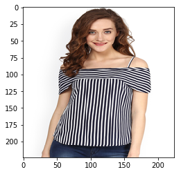
plt.imshow(q[0])
plt.show()
plt.close('all')
count = []
fig1 = plt.figure(figsize=(6,120), dpi=150)
for i in range(512):
ax1 = fig1.add_subplot(120,8,i+1)
t = intermediate_output[0][:,:,i]
if(np.sum(t)==0):
count.append(i)
ax1.imshow(t,interpolation='none',cmap="gray")
plt.axis('off')
pass
plt.show()
print("Number of zero filter : "+ str(len(count)))
Output shape : (1, 14, 14, 512)
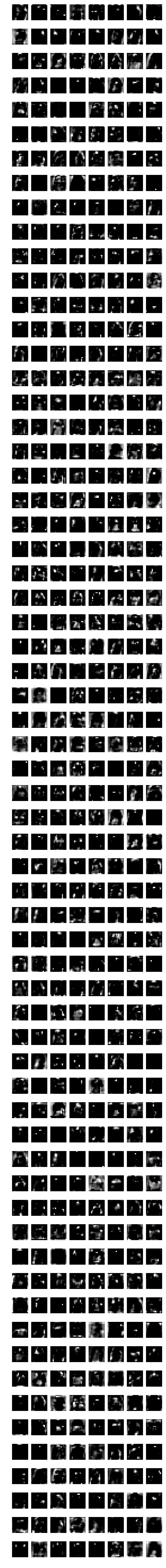
Number of zero filter : 15
Such intermediate representations help a tonne in debugging your network.
Conclusion
Now, that we have a model that is capable of generating good embeddings we are almost done. I will conclude this Visual Search series in the next post after sharing my results, inferencing logic and some other code snippets. Comment below to share any problems you are facing while implementing or training your visual search models.